Unveiling the Hydrological Symphony: Analyzing Short, Intense Storms in the Face of Climatic Shifts

Hello, I’m Dor, holding a B.Sc in Water Engineering. I’d like to share a segment of my final project, where I endeavored to predict the likelihood of intense storms. The data I gathered revealed some intriguing findings. For my final project, I utilized the Python programming language to extract rainfall data obtained from the Israeli Meteorological Services API. Throughout Israel, various gauges are strategically placed, and I specifically focused on data from digital gauges all over Israel. The gauges are on average with 20 years of measurements. Allow me to present a noteworthy observation (AMS- annual maximum series of the intensity of a 10 minutes duration storm) from the Tel Aviv Coast gauge data and delve into the statistical analysis derived from the information I collected. I’ll also discuss the connections between these findings and climate change.
In Figure 1, the Y-axis vividly illustrates the rain intensity measured in millimeters per hour during a concise 10-minute storm event. Meanwhile, the X-axis is dedicated to representing the annual probability of encountering the same or higher intensity event. This graph seamlessly introduces us to another significant and closely related concept: the Return Period.
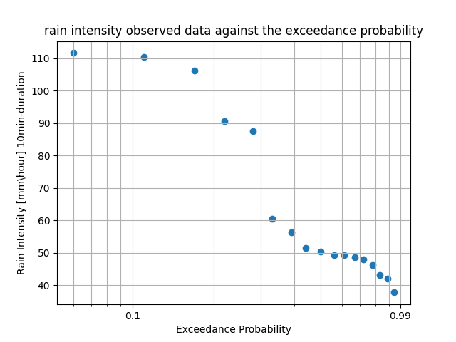
Figure 1: rain intensity observed data against the exceedance probability
This measure serves as a statistical gauge, estimating the average time between occurrences of a specific magnitude of events or those of a similar or higher intensity. The use of a return period expresses the level of risk and reliability of the system in dealing with extreme events. For example, an engineering structure built according to a flood event that will happen once every 100 years on average will have a probability of failure of 0.01 and hence a reliability of 0.99 (eq 1) [1]. For calculating the probability i used the ‘Plotting Position’ method. (eq 0).
eq 0.
\[\text{Probability} =\frac{\text{rank}}{n + 1}\] \[\text{Where } n \text{ is the sample size}\]eq 1.
\[\text{Reliability} = 1 - \text{Probability}\]However, it is crucial to remember that the return period is an average expression, signifying that one occurred event every 100 years on average does not eliminate the possibility that the event will occur again in two or three consecutive years later. In the context of our rainfall example, the Return Period provides valuable insights into how often we can anticipate storms of similar or higher intensity to take place over a given period. For instance, if the graph indicates a 5% probability for a particular rainfall intensity, the corresponding Return Period would be the reciprocal of this probability, suggesting that we can expect such a storm, or even more intense ones, on average, once every 20 years (eq 2).
eq 2.
\[\text{Return Period} = \frac{1}{\text{Probability}}\]The visualization of both probability and Return Period allows us to grasp the frequency and potential impact of these events, aiding in informed decision-making for urban planning, infrastructure resilience, and disaster preparedness.
The data spans from 2005 to 2022 and is arranged from the highest to lowest occurrences. Notably, the last five instances of the highest rainfall events transpired within the last seven years [Table 1]. This raises concerns about what the future may hold in terms of hydrological flood events and climate change.
Table 1: the data over the span of 2005-2022 from (spetember to september for each value) for a 10 min duration storm.
| Rank | Rain Intensity [mm/hour] | Year occurred | Probability | Return Period [years] |
|---|---|---|---|---|
| 1 | 111.6 | 2020-2021 | 6% | 18 |
| 2 | 110.4 | 2017-2018 | 11% | 9 |
| 3 | 106.2 | 2019-2020 | 17% | 6 |
| 4 | 90.6 | 2015-2016 | 22% | 4.5 |
| 5 | 87.6 | 2014-2015 | 28% | 3.6 |
| 6 | 60.6 | 2021-2022 | 33% | 3 |
| 7 | 56.4 | 2010-2011 | 39% | 2.6 |
| 8 | 51.6 | 2005-2006 | 44% | 2.25 |
| 9 | 50.4 | 2009-2010 | 50% | 2 |
| 10 | 49.2 | 2006-2007 | 56% | 1.8 |
| 11 | 49.2 | 2011-2012 | 61% | 1.6 |
| 12 | 48.6 | 2013-2014 | 67% | 1.5 |
| 13 | 48 | 2008-2009 | 72% | 1.4 |
| 14 | 46.2 | 2018-2019 | 78% | 1.3 |
| 15 | 43.2 | 2007-2008 | 83% | 1.2 |
| 16 | 42 | 2016-2017 | 89% | 1.125 |
| 17 | 37.8 | 2012-2013 | 94% | 1.05 |
Methodologies And Results
For the methodology part, I will show you what type of tests and tools I used. I used statistical analysis with the data in Python (SciPy), I was trying to find the best fit for this set of the observed data (AMS) I used the function ‘genextreme.fit’ to find out the parameters of the General Extreme Value (GEV) distribution Location, Scale and Shape.
input:
1
2
3
4
5
data = np.array([37.8, 42, 43.2, 46.2, 48, 48.6, 49.2, 49.2, 50.4, 51.6, 56.4, 60.6, 87.6, 90.6, 106.2, 110.4, 111.6])
loc, scale, shape = genextreme.fit(data)
print(f'Estimated Location: {round(loc,2)}')
print(f'Estimated Scale: {round(scale,2)}')
print(f'Estimated Shape: {round(shape,2)}')
output:
1
2
3
Estimated Location: -0.53
Estimated Scale: 49.28
Estimated Shape: 11.49
After finding those parameters I plotted the data with the probability density function (eq 3)
eq 3.
for $c = \xi$
\[\text{} f(x,c) = e^{-(1 - cx)^{\frac{1}{c}} (1 - cx)^{\frac{1}{c-1}}}\]$ \text{Where: } -\infty < x \leq \frac{1}{c} \quad \text{ if }\quad c > 0; \text{ and }\quad \frac{1}{c} \leq x < \infty \quad\text{ if }\quad c < 0; $
on figure 2 with the observed rain data on the x-axis and the density of the data on y-axis with the histograms and the PDF in the red line.
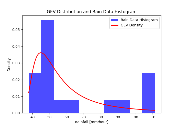
Figure 2: Is the rain data histogram with the fitted GEV distribution (PDF) function.
same thing did with normal distribution (figure 3)(eq 4).
eq 4.
\[\text{} f(x|\mu,\sigma) = \frac{1}{\sqrt{2\pi}\sigma} \cdot e^{-\frac{(x - \mu)^2}{2\sigma^2}}\]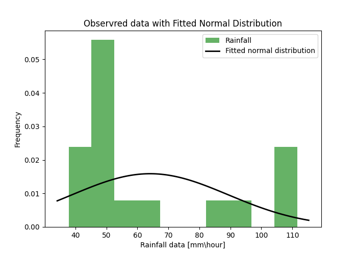
Figure 3: rain data histogram with the fitted normal distribution (PDF) function
After comparing figure 2 to figure 3 it was clear that a better fit for the set of AMS is GEV distribution.
figure 4 is the Cumulative Density Function (CDF) in red (eq 5) with the cumulative probability values for the data on the y-axis, and on the x-axis the values are quantiles of the data.
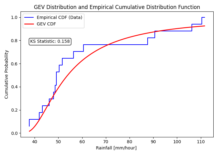
Figure 4: is the GEV distribution CDF with the ECDF of the data for the KS-test result
eq 5.
\[F(x; \mu, \sigma, \xi) = e^{ \left( -1 + \xi \left( \frac{x - \mu}{\sigma} \right) \right)^{\frac{-1}{\xi}} } \quad \text{for} \quad \xi \neq 0\]$\text{Where: } F(x; \mu, \sigma, \xi)\text{ is the CDF of the GEV distribution at point x}.$
$ \mu \text{ is the location parameter} $
$ \sigma \text{ is the scale parameter} $
$ \xi \text{ is the shape parameter} $
In this analysis, I conduct statistical test such as Kolmogorov-Smirnov (KS) which quantifies the maximum absolute distance between the empirical CDF (eq 6)
eq. 6
\[D = \max_{i} |F(x_i) - S(X_i)|\\\]Where: $S(x_i)$ is the empirical distribution function (EDF) at the $i\text{-th data point.}$
\[S(x) = \frac{\text{Number of data points} \leq x}{\text{total number of data points}} \text{}\\\]Where: $F(x_i)$ is the theoretical cumulative distribution function (CDF) $i\text{-th data point}$
of the GEV function (eq 3) to the distribution function that has been tested. That test compares the overall fit of distributions.The same method was applied with normal distribution (figure 5).
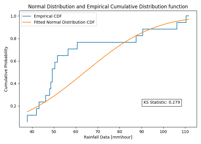
Figure 5: normal distribution CDF with the ECDF of the data for the KS-test result
It becomes evident that the most fitting correlation for this dataset is the “Generalized Extreme Value”, with a result of 0.158 in KS test (smaller result means less distance- better fit).
I wanted to conduct further analysis of the data, so I downloaded HEC-SSP (Hydrologic Engineering Center-Statistical software program), with that software I was able to see that on a product moment fitting method, the KS value was 0.184 for exponential distribution. (Table 1)
Table 2: Log results from the HEC-SSP analysis:
| Distribution | Parameter | Kolmogorov-Smirnov (Test Statistic) |
|---|---|---|
| Pearson III (PM) | Mean=64.094, StDv=25.888, Skew=1.018 | 0.227 |
| Gumbel (PM) | Loctn=52.443, Scale=20.185 | 0.236 |
| Shifted Gamma (PM) | Shape=3.857, Scale=13.181, Shift=13.250 | 0.227 |
| Generalized Pareto (PM) | Loctn=32.119, Scale=40.378, Shape=0.263 | 0.185 |
| Empirical (PM) | User-defined | NaN |
| Normal (PM) | Mean=64.094, StDv=25.888 | 0.274 |
| Generalized Logistic (PM) | Loctn=NaN, Scale=NaN, Shape=NaN | NaN |
| Triangular (PM) | Left=27.483, Peak=27.483, Right=137.317 | 0.197 |
| Uniform (PM) | Left=19.255, Right=108.934 | 0.245 |
| Beta (PM) | Shape0=NaN, Shape1=NaN | NaN |
| Gamma (PM) | Shape=6.130, Scale=10.456 | 0.237 |
| Exponential (PM) | Scale=64.094 | 0.446 |
| Generalized Extreme Value (PM) | Loctn=52.552, Scale=20.735, Shape=0.021 | 0.237 |
| Log-Logistic (PM) | Scale=59.913, Shape=4.956 | 0.265 |
| Ln-Normal (PM) | MeanLn=4.093, StDvLn=0.366 | 0.247 |
| Logistic (PM) | Loctn=64.094, Scale=14.273 | 0.294 |
| Shifted Exponential (PM) | Scale=25.888, Shift=38.206 | 0.184 |
| Log-Pearson III (PM) | MeanLog=1.778, StDvLog=0.159, Skew=0.785 | 0.206 |
| 4 Parameter Beta (PM) | Shape0=NaN, Shape1=NaN, Left=NaN, Right=NaN | NaN |
| Log10-Normal (PM) | MeanLog=1.778, StDvLog=0.159 | 0.247 |
Selected Distribution: Shifted Exponential (PM)
| Parameter |
|---|
| Scale=25.888136 ,Shift=38.205982 |
| Kolmogorov-Smirnov |
|---|
| 0.184 |
Conclusions
As we delve into the intricate patterns of hydrological events, The results between the data presented here to the fitting distributions, showcasing short but intense storms with high precipitation rates, of rainfall occurrences in the last 18-years had the best fit of GEV distribution as we saw in figure 2, high density among the entire data set of 110 mm\hour rain intensity event. This calls for a heightened awareness of the potential consequences that await us in the future. As we navigate these challenges, It seems there alot more of understanding to explore with the interconnectedness between the rising temperatures [2] to those extreme rain events that suddenly occurred in the last few years. In essence, the data serves not only as a record of the past but as a compass guiding us toward informed decisions for a more resilient future. It is our collective responsibility to address the implications of extreme rain events and strive for a harmonious coexistence with our ever-evolving environment. In my next posts, I will look at some of the temperature data and the correlation with extreme rain events.
Citations
[1] Vogel, Richard M., and Attilio Castellarin. “Risk, reliability, and return periods and hydrologic design.” Handbook of applied hydrology (2nd ed.)(pp. 78.1-78.10). New York, USA: McGraw-Hill Education (2017).
[2] Climate.nasa.gov global temperature data
Contact
👈👈👈 Let me know what you think of the work i did here, all my contact info on the left.